MATLAB: Thermal Systems Part 1

On Friday April 1st, we used MATLAB to model the heating and cooling of a cup of coffee under different conditions. We took the following expression that gives the temperature of a system exposed to air as time passes.

where dT = a small change in temperature

C = heat capacity

T = Current temperature

Tair = Temperature of the surrounding air

Rth = Thermal resistance

dt = a small change in time

Question 1:

How does the cooling behavior change if we vary the parameters and C? Figure this out using intuition and the above equations, and then vary these parameters in your program to confirm your conclusions.

Rearranging the above equation, T = Tair - (dT/dt) *(RthC). T is proportional to Rth and C. Therefore, increasing Rth would increase T as would increasing C. But we can also see from this same equation that dT/dt is inversely proportional to Rth and C. So with larger Rth or larger C values the change gets steeper. And smaller Rth and C values give a curve with smaller slopes at different parts. 

To test this, we modified the following code as noted in the comments and got the following results:

C = 100; Rth = 0.85

C = 10000; Rth= 0.85
Here, the temperature has shifted upwards (as expected, since C*Rth increased). But the slope over each small time interval has significantly decreased.  

C = 1000; Rth = 0.085
Here, you can see that the graph resembles the C = 100; Rth = 0.85 graph. This shows that it is  really the product of C and Rth that affects the slope. 

We intentionally chose values of Rth and C dramatically different from the original values to see the change clearly. 

Question 2: Calculate a good value for P if we want our coffee to heat up to the Starbucks ideal 84°C, using the Rth from the MATLAB script?

This time, we considered a system where the coffee is sitting on a heating plate that provides a power of P. We used the following expression to find the value of P that would heat up the coffee to 84°C.

P = (dT/dt)C + (T-Tair)/Rth; where Rth = 0.85

But at t = 0, dT/dt = 0. So P = (T-Tair)/Rth = (84 - 20)/0.85 

P = 75 J/s

From the following graph deduce the thermal parameters C and Rth:

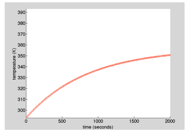
From the relation,  P = (change in T) / Rth, we can rearrange to get Rth = (change in T) / P, which in this case is about (350 - 290) K / 75 Watt = 0.8 K/Watt.

From dT/dt = P/C at t = 0, we can rearrange to get C = P/(dT/dt)

If you focus on the first part of the curve near t = 0, it resembles a line with a slope of 20/250 = 1/12.5

Therefore C = 75 W * 12.5 s/K = 937 J/K ~ 1000 J/K, which is the given value. My values are a little off because we can only make estimates from the graph.  

Question 3: Simulate a temperature controller that uses bang-bang control to reach and maintain the desired temperature. Bang-bang control is a very common approach for thermostats. 

We used the following script:

And we got the following graph:

After T = 357 the curve starts oscillating very subtly. This is because the power turns off when the temperature exceeds 357 K  and turns on when it drops below this desired value. Since it always overshoots the goal a little bit, some oscillation is expected but since the temperature stays very close to 357 K, the coffee will still be very close to the desired temperature, and certainly not much hotter or colder. 

Why is bang-bang control appropriate for many thermal systems? When might it be insufficient?

Thermal systems like this one can be adjusted to a good enough precision to maintain a certain temperature. The small fluctuations in temperature as the system continuously adjusts its output keep systems like thermostats at reasonably close temperatures to the desired value. This might be insufficient if a very precise constant temperature is desired or if one needs a continuous and shift in temperature as a reaction to a drop or increase in the measured. 

Question 4: Create a program that uses proportional control to reach and maintain the desired temperature. How does this approach compare to bang-bang control?

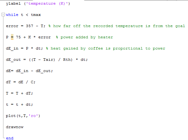
We used the following script:

 And we obtained this graph:

This graph appears a lot smoother and the value of the final temperature constantly approaches 357 instead of oscillating between values slightly above and below this point (unlike bang-bang control). This is because the power supplied to the coffee decreases linearly as the temperature approaches the goal. So, we prevent overshooting the goal and having to come back for it. 

This gives a more steady and precise temperature. It is also easier to reach the desired temperature in a short amount of time. 

Question 5) Suppose there is a delay between the time the coffee reaches a given

temperature and when the temperature sensor records that temperature. Modify

both of your programs to include this effect, along the lines of the programs on the next few pages that I showed in class, which explore the effect of adding a “sensor delay” to a simulation of moving a SciBorg lego car a particular distance. 

Here are the bang-bang and proportional control codes respectively that account for the delay (chosen to be 5 seconds here).

Bang-Bang Control with delay:

Proportional control with delay:

This yielded: 

Proportional control with a delay of 5

This graph shows a brief oscillation before it flattens at around 355.

What other might you expect in your thermodynamic system, apart from sensor delays?
I would expect a delay in heat transfer. Since radiation goes at the speed of light and everything else at a lower speed, there is always a time lag between heat loss or gain by the coffee.
In addition, the actuator itself would have a lag between it receives the "order" to turn on the power supply and when it actually does.

MATLAB Introduction

On Tuesday, March 29th, we started our introduction lesson to MATLAB by reading the first 4 chapters of "Physical Modeling in MATLAB" by Allen B. Downey and completing the following exercises.

Exercise 2.1: Fibonacci1 Script
The goal of this exercise was to calculate the nth term in the Fibonacci sequence that has the form, F(n) = F(n-1) + F(n-2) where F(1) = 1, F(2) = 1. In other words, every term (starting from the third) in this sequence is the sum of the two terms before it. We used the following expression to find the nth term. We wrote the program such that when we run the code, it asks us to enter a value for n and then prints the value of Fn.

Code and Results:

This exercise helped train us write mathematical expressions the way MATLAB understands them.  As you can see, n = 10, for example gives us the correct Fn value of 55.

Exercise 2.3: car_update script
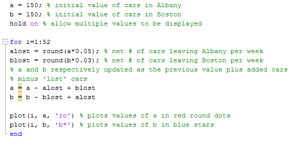
In this exercise, we pretended we had a car rental company with a branch in Boston and another in Albany. Customers can pick a car from either location and drop it off at either location. We are told that initially there are 150 cars in each location and 5% of the cars from Albany end up Boston while 3% of the cars from Boston end up in Albany every week. We wrote a script that updates the number of cars in each location every week.

We represented total number of cars left in Albany with the letter a and those in Boston with the letter b.

Script and results:

Exercise 3.1 and 3.2: car_loop script with plotting
(also trying values of a and b = 10000)
The previous code required us to manually enter each value of a and b to get the next pair. This is a bit tedious especially when dealing with a large amount of data. So this time, we created a loop that runs the above functions of a and b 52 times and helps us see if the values increase, decrease, oscillate or approach a constant.

Here are the first few values the loop produced: 

We also plotted it to see this pattern.

 For initial values a = 150 and b = 150


For initial values of a = 10000 and b = 10000

 It is interesting that the 10000-cars curve is smoother at the bend towards its constant value.

For starting values of a = 150 and b = 150, we get constant values a = 116 and b = 184 after the 24th week. The number of cars left in Albany decreases and that in Boston increases until they reach these constant values.

Exercise 3.5: fibonacci2 sequence script
Here we used a for loop to make MATLAB give us the 10th and later the more general nth number.

Scrips and results:

• Exercise 4.6: plotting fibonacci ratios
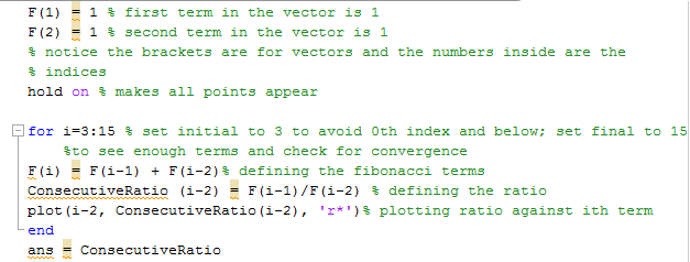
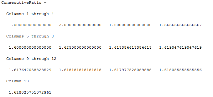
After learning about vectors and plotting techniques in Chapter 4, this exercise challenged us to write the Fibonacci sequence as vector, another vector with the ration of the consecutive numbers in the Fibonacci sequence and plot the latter to see if the ratio converges.

Scripts and results:

 

 The ratio converges to 1.618 after the 7th term.

Sci Borg Part 3

In the word of an engineer friend, proportional control is like working with a spring. For fellow physics enthusiast, F = -kx is a familiar expression that relates the force acting on an object attached to a spring (without damping) due to a displacement. The magnitude of the force increases (linearly) as the distance x increases. And k is the constant of proportionality that relates them.

Very similarly, we can use proportional control to change the behavior of our SciBorg (analogous to force) based on a change or error (analogous to displacement) recorded by a sensor. 

In the third part of our SciBorg project, we related the speeds of the motors to a linear expression containing k*error to:

              I) Drive Straighter

              II) Travel 10 ft and stop

              III) Follow an object using an ultrasonoic sensor

              IV) Follow a line using a light sensor 

I) Driving Straighter Using Proportional Control

We set a base speed of 150 to both motors and changed the speed of Motor 1 based on the relation v1 = 150 + error * k, where error = encoder reading for motor 2 - encoder reading for motor 1, and k is an arbitrarily set constant of proportionality that we changed based on observations.

Below are the sketch used, the different k values tried and their serial port readings, as well as videos showing how the SciBorg performed on the lab floor, a carpet, when the wheels traveled on surfaces of different friction constants, and going up/down a ramp (we have yet to try because the ramp is not set up now).

The results over several trials were fairly constant. The car looked less shaky than it did in the bang-bang control partly because proportional control results in gradual changes rather than abrupt turns.

 Sketch:

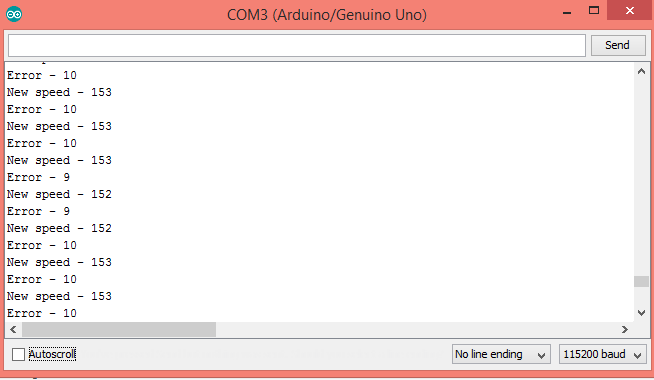
K=0.1

K=0.3

K=0.5

On the lab floor:

On a carpet:

With wheels on different surfaces:

Notice that the wheel on the smoother surface always moves faster and the car turns to the side away from this smooth surface. This is because we calibrated our k and our motor speeds for a surface where both wheels face the same amount of friction.

II) Go 10 feet

We used a similar logic of making the speed linearly dependent on some changing variable. But this time, we made the speed dependent on the number of encoder readings the car needs to go before it reaches its destination. This number of counts left decreases as the car approaches its destination, so it slows down before it finally stops. 

First, we attempted to find the encoder reading after the car has traveled 10 ft by timing the car travel the 10 ft and then timing the encoder reading as it is attached to the serial monitor. Later, we figured where we recorded encoder values and where we ran the car are different environments in which friction and power supplied to motors varies (the computer actually provides additional energy to the motors). 

Instead, we decided to calculate the number of encoder counts per rotation, which should be a constant value because the encoder readings come from physical structures within the motor.

We conducted the following mini experiment, where we took the ratio of the wheels' circumference to 10 ft and the encoder readings per turn to find the encoder readings per rotation.

(I will provide a more organized version of this picture with more time.)

Below are the sketch used and the video of Daniela (our SciBorg) stopping after traveling ~10 ft on the lab floor. 

Notice the tail not the front of the car was on the start line and it stops very close to 10 ft from where it starts (less than 3 in of uncertainty). However, we also attempted to use the nudge function.

Sketches and video below:

Ideally, we would have used a relation that looks like speed = k * counts left. However, when the speed is really small, the car starts wobbling and changing direction. It also stops before speed is actually equal to zero. So the function of our proportional control ended up being mostly slowing the car down before we tell the motors to stop. 

III) Using ultrasonic sensor follow objects
In this section we made the speed of the motors dependent on the distance of an object from the ultrasonic sensor. Given the relation, speed = 170 + k*error, the speed increases with a positive error and decreases with a negative error.

Again, because lower speeds result in an unstable SciBorg, we used the proportional control as a means of slowing the car down before it stops.

This worked well as the Daniela followed my feet and then other SciBorgs. I would say this worked as well as the bang-bang control method, especially because the stopping distance not precise as long as the SciBorg followed others and stopped before crashing into the object.

In this last video, Daniela was the one at the back.

IV) Proportional line following 

We faced the most challenge in this one because, while the logic made sense, the result was completely unpredictable.
Our setup:
We placed the sensor to the left of the line and told the code to set speed of motor 1 to 150 + k*error, where error = value of brightness - 80. We took 80 because it was the reading right between the brown and the white surfaces.

With error > 0 speed of motor 1 should increase, therefore car turns towards motor 2; error < 0 speed of motor 1 should decrease, therefore car turns towards motor 1.

In practice, this didn't happen.

Here are some of the several loop commands we attempted:

And when this didn't work:

In some of these cases the car just went straight ahead, while in others it just turned to the right.

Expect to hear back from me on this one.

Real World Feedback and Control

Feedback and control systems are more familiar than their fancy name makes them sound. A large range of objects, from automatic doors and faucets to drones and spaceships rely on feedback and control systems. 

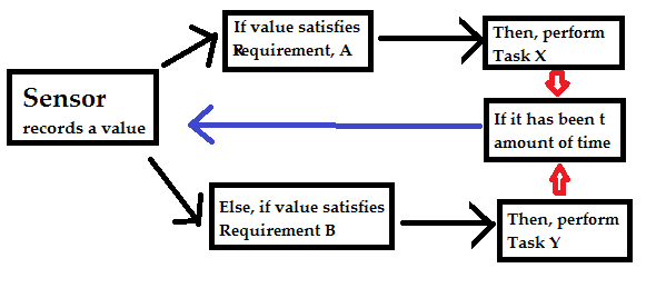
These systems have sensors, computers, and actuators that change the behavior of the machine based on observed light, movement, sound, heat, interference, etc. The control system, for example, can use if/else statements to make the machine behave one way when its sensor observes a specific property in its surrounding and to act differently otherwise. 

The diagram above shows the general mechanism by which feedback and control systems work.

In class, we have seen two types of feedback and control systems -- open and closed loop. We have also used light sensors, ultrasonic sesnsors, encoders, and switches in combination with Arduino sketches to change and control the behavior of SciBorgs. 

Below, I present four common feedback and control systems I encounter daily: automatic doors, automatic water dispensers and faucets, automatic phone operators and smoke detector alarms. 

1) Automatic doors 

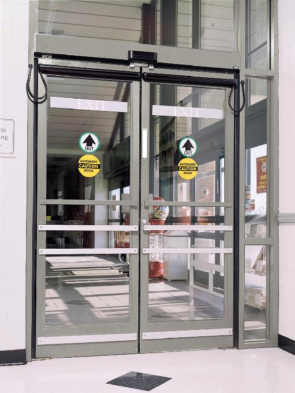
Such doors use light sensors, touch switches, or other sensors to open doors for a given amount of time in response to an observed change in the surrounding. 

PIR Sensor

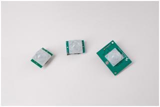
Some automatic doors use PIR (Passive Infrared Sensor) to detect the presence of humans. The near-black-body irradiation from our body due to our temperature is mostly in the form of infrared waves (~9500 nm). And the intensity (or the number of photons reaching the sensor) increases with shorter distance between the source and the detector. So the intensity of IR photons detected by the sensor on an automatic door increases when a human is near the sensor. The PIR has a crystal whose temperature increases upon irradiation (by the IR waves reaching it). This temperature creates an electric signal/charge that communicates with the micro-controller. The micro-controller orders the motors and other actuators in the system to move such that the door opens when there is a high IR signal (or change thereof) and close after a certain delay, and remain closed when the IR signal is low in terms of intensity: the person is far; or in terms of temperature: the radiation reaching the sensor is only that of the surrounding inanimate materials. 

Note: This sensor is called "passive" because unlike ultrasonic sensors, for example, it doesn't send out waves and measure the time delay before they return to observe something about the surrounding. It simply detects input from the environment. 

This has the following uses: 

•  If a person cannot open the door due to a disability, because their hands are full, or they are too weak to do so (for example, a child), it is convenient to have an automatic door that doesn't need force to open.
• Since the amount of time the door stays open is controlled, it avoids the risk of leaving the door open for too long and wasting either heater or AC energy.

Some drawbacks:

• Since the specific sensor I discussed only detects IR reaching it an not the identity of the emitter, it can let either animals or children in our out the of the building without adult supervision. 
• It adds to the load of power use by the building. We would spend more energy on doors than we would if we manually opened them. But often this drawback is overcome by the many advantages of such systems. 

2) Automatic faucets

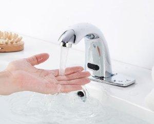
Automatic faucets can also use PIR but since one might want to wash items with temperatures lower than that of humans, such faucets also use ultrasonic sensors or infrared light next to a an IR detector to "measure the presence" of an item within a predefined distance. The object interrupts a light beam from the ultrasonic or the IR source and which reflect back to the sensors. If the reflection time is in the range of the calibrated value for a hand under the faucet (AKA not the sink or other items in the surrounding), an electric signal is sent to a solenoid valve (an electromagnet) to turn on the faucet. Otherwise, the solenoid valve isn't activated and the faucet remains closed. 

Advantages: 

• It prevents water waste because if a person forgets to close the faucet, the IR or ultrasonic interruption is no longer present and the faucet turns off instantaneously
• It is also sanitary especially in public bathrooms where manually opening faucets may introduce us to several germs. 

Drawbacks: 

• The specific systems described above don't allow the user to choose the water temperature. 
• While we save a lot of water, we have to sacrifice some electrical power. 

3) Ionization Smoke Detectors/Alarms

Smoke detectors contain a very tiny amount (on the order or 10^-6 g) of Americium which decays radioactively and emits alpha particles. These alpha particles collide with the nitrogen and oxygen molecules in the air and trigger a current flow in the opposite direction to an original current that would activate an alarm. This means the net current flow when there is ample N2 and O2 in the air is zero; the alarm can't go off. However, when smoke blocks off the clean air from occupying the space near the detector, not enough charges are created to counter the current that triggers the alarm. And depending on the occasion, either a life is saved or the user rushes to wave a towel under the detector (that is how my roommate and I handle completely random alarms). The following video from YouTube offers a good explanation for how this feedback and control system works: 

Advantages:

• The detector is very sensitive and gives a very early warning to the start of fire before too much damage happens. Also because smoke detectors sit on top of the room, hot air from the fire reaches them quickly through convection. 
• Needless to say, they save lives.
• While the radioactive material sounds dangerous it poses little threat due to its small amount and proper packaging.

Drawbacks:

• Disposal of smoke detectors containing radioactive material can be a health and environmental hazard if not done properly. 
• There is a chance the alarm would go off even though there is no risk of fire. It is so sensitive, steam or dust can set it off sometimes. This is because it detects the absence of ions rather than the specific material that is present in their stead. 

4) Fume Hoods

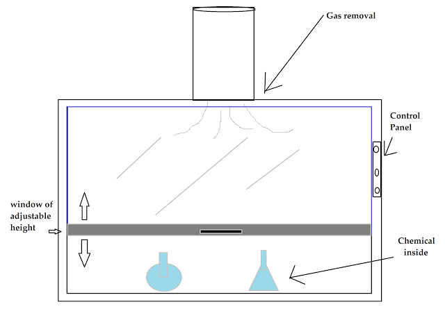
Fume hoods are "cupboards" that enclose a working area to isolate and remove harmful gases from the room in which a chemist (mostly) works. They have feedback and control systems that monitor air flow and window height (opening), as well as allow the user to turn exhaust fan on and off. 

Fume hoods have an air flow monitor that detects the face velocity (velocity of air at the fan opening). When the detected air flow is too low either due to excess exhaust, the sash being opened too high, or fan malfunction, an alarm goes off.

Advantages: 

• Not only does it do the primary job of pumping out unwanted gas and replacing it with fresh air, it assesses the product: how high the air flow is. 
• It prevents health and environmental hazards while allowing us to work with a variety of chemicals

Disadvantages: 

• It runs for several hours and pumps out air from the room that has been thermally conditioned. So it ends up consuming too much energy.